NAMD计算
记录计算NAMD过程的一些笔记以及注意事项(只记录计算步骤,不涉及背后原理,因为我自己也没搞明白,后续可能会有完善)
基于凯峰给的NAMD-example
NAMD_example
    Mode                 LastWriteTime         Length Name
    ----                 -------------         ------ ----
    dar--l        2024/12/10      0:52                NA_couplings
    dar--l        2024/12/10      0:52                step1
    dar--l        2024/12/10      0:52                step2
    dar--l        2024/12/10      0:52                step3
    dar--l        2024/12/10      0:52                vasp.5.4.4-nac-intel
    -a---l        2022/11/19     10:39            390 readme
NAC计算大致分为三步
- 跑MD(包括heating部分和MD部分)
- 将MD获得的轨迹分割成5000个POSCAR,并对每个POSCAR进行一遍scf(pyxaid一定要单k点跑)
- 计算寿命,退相干
其中NA_couplings包含计算所需脚本及可执行文件
Step1,进行vasp的MD计算
heating
step1下包含heating和MD
 $ ls
heating  MD
MD过程包含heating和MD两个部分
heating过程主要使结构在300K下跑1000步(或者500步),并写入WAVECAR,INCAR设置如下:
SYSTEM  = crystal
#ISYM = 0
ENCUT   = 500 #和先前计算保持一致
LREAL = A
ISTART  = 0
ISYM = 0
NELM = 200
NPAR    = 6
ICHARG  = 2
ISMEAR  = 0 #feimi 0 gass
SIGMA   = 0.02
EDIFF   = 1E-4 #can be modified
NBANDS  =  846 # should be modified grep NABNDS OUTCAR
PREC    = M    # Low | Medium | High | Normal | Accurate | Single
##################### MD  Ionic Relaxation#######################
IBRION=0      #(df:0/(-1 if NSW=0/1))relax method,non:-1,MD:0,CG:2.
POTIM=1.0     #(df:0.5)controll the length of the trial step for ionic relax.
ISIF=2        #(df:2)Control what to relax. usually:0,all:3.
NSW=1000       #(df:0)max. ion relax steps.
EDIFFG=-0.01  #(df:EDIFF*10)ionic rel. brake cond. loop force:(-),Ener.(+)
NELMIN=6      #(df:2)minimum steps of electronic SC.
ALGO = N        # FAST is faster than Normal
NBLOCK = 4
TEBEG=300
TEEND=300
SMASS=-1      #-1 heating;-3 normal MD.controls the velocities during an ab-initio molecular dynamics

######################Write Flags############################
LWAVE   = .T.
LCHARG  = .FALSE.
IVDW    = 12
NWRUTE  = 1
根据自己需求可以适当修改,使用vasp_gam进行计算
MD
MD过程的POSCAR为计算完heating的CONTCAR,且需要读取heating的WAVECAR
ICNAR设置如下:
SYSTEM  = crystal
#ISYM = 0
ENCUT   = 500 #和先前计算保持一致
LREAL = A
ISTART  = 1
ISYM = 0
NELM = 120
NPAR    = 8
ICHARG  = 2
ISMEAR  = 0 #feimi 0 gass
SIGMA   = 0.02
EDIFF   = 1E-4 #can be modified
#NBANDS =  856 # should be modified grep NABNDS OUTCAR
PREC    = M  # Low | Medium | High | Normal | Accurate | Single
##################### MD  Ionic Relaxation#######################
IBRION=0      #(df:0/(-1 if NSW=0/1))relax method,non:-1,MD:0,CG:2.
POTIM=1.0     #(df:0.5)controll the length of the trial step for ionic relax.
ISIF=2        #(df:2)Control what to relax. usually:0,all:3.
NSW=5020       #(df:0)max. ion relax steps.
EDIFFG=-0.01  #(df:EDIFF*10)ionic rel. brake cond. loop force:(-),Ener.(+)
NELMIN=6      #(df:2)minimum steps of electronic SC.
ALGO = N        # FAST is faster than Normal
NBLOCK = 1
TEBEG=300
TEEND=300
SMASS=-3      #-1 heating;-3 normal MD.controls the velocities during an ab-initio molecular dynamics

######################Write Flags############################
LWAVE   = .F.
LCHARG  = .FALSE.
IVDW    = 12
MD过程NSW离子步设置为5020,使用vasp_gam计算
计算完成后,需要将MD的轨迹拆分为一个一个POSCAR,可以使用脚本实现。
轨迹文件在MD目录下生成的XDATCAR,脚本位于NA_couplings文件夹下的gxdatpos
需要将脚本和轨迹文件放入/step2/pfile/, 然后执行脚本拆分轨迹,获得所需的5020个结构
需要注意:MD跑完后一定要检查轨迹(导入至
VMD中),看看结构是否正常,否则后续跑NAMD没啥意义
接下来计算NAC
Step2,进行NAC计算(单K点!!!)
NAC计算非常耗时,成本高,一定要时刻注意是否计算正确,提交任务前一定要检查好参数,尤其是:
MINB=168   #一定要记得修改!!!
MAXB=177
一定要和EIGENVAL里面保持一致,在SOC或者扩胞后会有变化。
step2目录下,有如下文件:
 $ ls
combine_complex.py  NAC      pfile                 readme            real
energy              name.py  read-en-diff-vasp.pl  read-nac-vasp.pl  res
首先先计算NAC
NAC目录下,有如下文件:
 $ ls
FIRSTCAR  readme  nac.sh  STARTCAR
 $ cat FIRSTCAR
Step 1 adiabatic MD INCAR
ISTART=0
ALGO=N    #VASP relaxation algorithm
NELMDL=-2
LWAVE = .TRUE.
LCHARG = .FALSE.
LREAL = A
NPAR = 8
PREC=M
ISMEAR= 0         #set to 0 for partial occupencies of wavefunction have Gaussian smearing
SIGMA=0.02
ISYM = 0          #symmetry not considered in calculation
NSW=0
EDIFF= 1E-4
EDIFFG=-0.01
IVDW    = 12
 $ cat STARTCAR
Step 1 adiabatic MD INCAR
ISTART=1
ALGO=N    #VASP relaxation algorithm
NELMDL=-2
LWAVE = .TRUE.
LCHARG = .FALSE.
LREAL = A
NPAR = 8
PREC=M
ISMEAR= 0         #set to 0 for partial occupencies of wavefunction have Gaussian smearing
SIGMA=0.02
ISYM = 0          #symmetry not considered in calculation
NSW=0
EDIFF= 1E-4
EDIFFG=-0.01
IVDW    = 12
nac.sh脚本需要设置好路径,包括NA_couplings路径 pfile路径(有两处)
MINB:电子可以激发的最低能量轨道
MAXB:电子可以激发的最高能量轨道
一般MINB设置为VBM占据轨道减去4,MAXB设置为CBM占据轨道加上4(可以在本征值文件EIGENVAL查到) (换了体系或者加了SOC后,一定一定一定记得修改这儿!!!)
MINT和MAXT:起始步和结束步。(若要分段算最好第二段往前多算几步,比如1-2505;2500-5005)
注意自己是用的vasp_gam还是vasp_std
计算结束后检查energy文件行数和real文件夹中的real文件数是否是对的(多次计算生成的energy内容并不会被覆盖,而是会在末尾继续写入,一定要检查好)
然后cp energy和real文件到/step2/energy文件和real文件夹
 $ cat nac.sh
#!/bin/bash
#SBATCH -J ljb-nac              # 作业名
#SBATCH -o out.%j               # 标准输出文件(%j 为作业 ID)
#SBATCH -e err.%j               # 标准错误文件
#SBATCH -p mars                 # 分区名称
#SBATCH -N 1                    # 申请 1 个节点
#SBATCH --ntasks-per-node=64    # 每个节点 64 个任务
#SBATCH -t 07-23:57:25          # 运行时间限制 (7天23小时57分25秒)

# 加载必要的模块
module purge
module load intel/oneapi2023.2_noimpi
module load mpi/mpich/4.1.2-gcc-11.4.0-ch4

# 设置 VASP 路径
export PATH=/GLOBALFS/caep_lts_qrhzh_1/liaojinbo/soft/vasp.5.4.4-nac-intel/bin/:$PATH
module list

# 当前工作目录
cd $SLURM_SUBMIT_DIR

echo "ENV Load Done" > Debug.log

PATH=$PATH:/GLOBALFS/caep_lts_qrhzh_1/liaojinbo/soft/NA_couplings  # puts perl scripts in path
export $PATH
# 参数设置
MINB=168   #一定要记得修改!!!
MAXB=177
MINT=1
MAXT=5000
total_k=1
TMSTP=1.0

# 打印参数
printf "\n\n======= INITIAL PARAMETERS (MINBAND MAXBAND MINTIME MAXTIME) ========\n"
printf "%10d%10d%10d%10d\n\n" $MINB $MAXB $MINT $MAXT
rm -f billdata OS_STRENGTH in_SPECTRUM test_coupling_os coupling

echo "Set up Calcs Done" >> Debug.log

# 获取初始 POSCAR 文件
SUFX=$( printf "%04d" "$MINT" )
POSFILE="p${SUFX}"
cp ../pfile/$POSFILE POSCAR  #可以更改为相对路径,就不需要每次计算都改这里了
cp FIRSTCAR INCAR

# 执行 VASP 初始化计算
printf "Running VASP and getting initial set of good orbitals\n"
yhrun -N 1 -n 64 vasp_std > vasp.out 2> err
cat vasp.out >> Debug.log
cp WAVECAR WAVECAROLD
cp WAVECAR WAVECARNEW
cp OUTCAR OUTCAR_total

echo "Set Good ORBITALS Done" >> Debug.log

# 逐步计算 NAC
(( MINT++ ))

for i in $(seq $MINT $MAXT); do
    SUFX=$( printf "%04d" "$i" )

    POSFILE="p${SUFX}"
    cp ../pfile/$POSFILE POSCAR
    cp STARTCAR INCAR
    printf "Running VASP at t = $i fs\n"
    yhrun -N 1 -n 64 vasp_std > vasp.out 2> err
    cat vasp.out >> Debug.log

    mv WAVECARNEW WAVECAROLD
    cp WAVECAR WAVECARNEW
    cat OUTCAR >> OUTCAR_total

    printf "Getting band energies at t = $i fs\n"
    state_energy_extractor_allk.pl $MINB $MAXB
    cat energy_by_band >> energy

    # 计算 NAC
    echo "Calculating the NAC among k points" >> Debug.log
    yhrun -N 1 -n 16 ovlap_NORM_OS_allk_mpi $MINB $MAXB $TMSTP $total_k $SUFX >> Debug.log
    rm -f billdata OS_STRENGTH in_SPECTRUM test_coupling_os

    # 合并 real 文件
    for j in $(seq 1 $total_k); do
        mv "real${SUFX}_${j}_1" "real${SUFX}_${j}"
        for k in $(seq 2 $total_k); do
            paste "real${SUFX}_${j}" "real${SUFX}_${j}_${k}" > temp
            mv temp "real${SUFX}_${j}"
            rm -f "real${SUFX}_${j}_${k}"
        done
    done

    mv "real${SUFX}_1" "real${SUFX}"
    for j in $(seq 2 $total_k); do
        cat "real${SUFX}_${j}" >> "real${SUFX}"
        rm -f "real${SUFX}_${j}"
    done
done

echo "Combine the real files Done" >> Debug.log

# 将 real 文件移入目录
(( MINT-- ))
REALDIR="REAL_${MINT}_${MAXT}"
mkdir -p $REALDIR
mv real* $REALDIR/
echo "Finish" >> Debug.log
可以看到,NAC计算过程还是比较复杂的,在nac.sh脚本帮助下可以大大提高效率。
计算完成,会在当前目录下创建REALDIR="REAL_${MINT}_${MAXT}"目录,并将计算得到的real文件移动到此。
确保step2目录下含: combine_complex.py和name.py,如果没有res文件夹则mkdir res
使用combine_complex.py脚本在real文件夹中生成哈密顿量的实部和虚部,然后cp real文件夹的实部和虚部到res文件夹
接着运行name.py,将res文件夹中的文件顺序减2,运行cp.py(记得修改复制循环次数),当然也可以一键运行gennaccopy.sh,省的自己动手。(别忘了这一步,否则namd计算会报错)
获取带隙波动和NAC:可以将read-en-diff-vasp.pl和read-nac-vasp.pl脚本放到step2最终的res文件,执行这两个脚本得到en-diff.dat和nac.dat。(注意:nac.dat的数值需要取绝对值并算平均值。)
step3 获取Population,Dephasing和Spectral_density(基于Pyxaid)
step3包含如下文件:
total 329
    0 Dec 24 17:02 err.273230
11776 Dec 23 16:41 FFT
11776 Dec 24 17:00 macro
  916 Dec 23 16:41 name_new1.py
  916 Dec 23 16:41 name_new2.py
  916 Dec 23 16:41 name_new3.py
11776 Dec 23 16:41 out
 6146 Dec 24 17:02 out.273230
 8507 Dec 24 17:07 py-scr3.py
  811 Dec 24 17:01 pyxaid-slurm.sh
 1596 Dec 24 17:20 readme
12800 Dec 24 17:08 res
12800 Dec 24 16:59 res1
13824 Dec 24 16:59 res2
13824 Dec 24 16:59 res3
旧脚本
name_new.py作用为复制哈密顿文件并重命名,以5000为例,需要复制3次,得到3个res1,res2,res3。如,设初始res顺序为ABC,则经过脚本处理后res1为ABCBA,res2为ABCBC,res3为ABCAB,将res1、2、3中所有文件cp到新的res文件,会去掉相同的部分,最终得到ABCBABCBA。
使用
name_new.py需要python2.7版本,python3会报错不兼容。
py-scr3.py脚本(需要修改部分:i, i+namdtime要小于res文件的实部或虚部数量)res1,res2,res3,(为step2的res cp 的,对应与name_new(1,2,3).py脚本)
旧脚本
根据自己需求修改py-scr3.py
其中py-scr3.py内容为:
$  cat py-scr3.py
from PYXAID import *
#from pyxaid_core import *
import os

print('import Done')
#############################################################################################
# Input section: Here everything can be defined in programable way, not just in strict format
#############################################################################################
print('Init Params!')
params = {}

# Define general control parameters (file names, directories, etc.)
# Path to Hamiltonians
# These paths must direct to the folder that contains the results of
# the step2 calculations (Ham_ and (optinally) Hprime_ files) and give
# the prefixes and suffixes of the files to read in
rt =os.getcwd()
params["Ham_re_prefix"] = rt+"/res/0_Ham_"
params["Ham_re_suffix"] = "_re"
params["Ham_im_prefix"] = rt+"/res/0_Ham_"
params["Ham_im_suffix"] = "_im"
params["Hprime_x_prefix"] = rt + "/res/0_Hprime_"
params["Hprime_x_suffix"] = "x_re"
params["Hprime_y_prefix"] = rt + "/res/0_Hprime_"
params["Hprime_y_suffix"] = "y_re"
params["Hprime_z_prefix"] = rt + "/res/0_Hprime_"
params["Hprime_z_suffix"] = "z_re"
params["energy_units"] = "Ry"                # This specifies the units of the Hamiltonian matrix elements as they
                                             # are written in Ham_ files. Possible values: "Ry", "eV"

# Set up other simulation parameters:
# Files and directories (apart from the Ham_ and Hprime_)
params["scratch_dir"] =  os.getcwd()+"/out"  # Hey! : you need to create this folder in the current directory
                                             # This is were all (may be too many) output files will be written
params["read_couplings"] = "batch"           # How to read all input (Ham_ and Hprime_) files. Possible values:
                                             # "batch", "online"

# Simulation type
params["runtype"] = "namd"                   # Type of calculation to perform. Possible values:
                                             # "namd" - to do NA-MD calculations, "no-namd"(or any other) - to
                                             # perform only pre-processing steps - this will create the files with
                                             # the energies of basis states and will output some useful information,
                                             # it may be particularly helpful for preparing your input
params["decoherence"] = 1                    # Do you want to include decoherence via DISH? Possible values:
                                             # 0 - no, 1 - yes
params["is_field"] = 0                       # Do you want to include laser excitation via explicit light-matter
                                             # interaction Hamiltonian? Possible values: 0 - no, 1 - yes

# Integrator parameters
params["elec_dt"] = 1.0                      # Electronic integration time step, fs
params["nucl_dt"] = 1.0                      # Nuclear integration time step, fs (this parameter comes from
                                             # you x.md.in file)
params["integrator"] = 0                     # Integrator to solve TD-SE. Possible values: 0, 10,11, 2

# NA-MD trajectory and SH control
params["namdtime"] = 2000                      # Trajectory time, fs 计算步数,需要修改
params["num_sh_traj"] = 300                 # Number of stochastic realizations for each initial condition
params["boltz_flag"] = 1                     # Boltzmann flag (set to 1 anyways)
params["Temp"] = 300.0                       # Temperature of the system
params["alp_bet"] = 0                        # How to treat spin. Possible values: 0 - alpha and beta spins are not
                                             # coupled to each other, 1 - don't care about spins, only orbitals matter

params["debug_flag"] = 0                     # If you want extra output. Possible values: 0, 1, 2, ...
                                             # as the number increases the amount of the output increases too
                                             # Be carefull - it may result in a huge output!
print('Parameters of the field (if it is included)')
# Parameters of the field (if it is included)
params["field_dir"] = "xyz"                 # Direction of the field. Possible values: "x","y","z","xy","xz","yz","xyz"
params["field_protocol"] = 1                # Envelope function. Possible values: 1 - step function, 2 - saw-tooth
params["field_Tm"] = 25.0                   # Middle of the time interval during which the field is active
params["field_T"] = 25.0                    # The period (duration) of the field pulse
params["field_freq"] = 3.0                  # The frequency of the field radiation = energy of the photons
params["field_freq_units"] = "eV"           # Units of the above quantity. Possible values: "eV", "nm","1/fs","rad/fs"
params["field_fluence"] = 1.0               # Defines the light radiation intensity (fluence), mJ/cm^2

print('Params Done!')

# Define states:
# Example of indexing convention with Nmin = 5, HOMO = 5, Nmax = 8
# the orbitals indices are consistent with QE (e.g. PP or DOS) indexing, which starts from 1
# [ 1, 2, 3, 4, 5, 6, 7, 8, 9, 10, 11] - all computed orbitals
# [ 1, 2, 3, 4, 5, 6]                     - occupied orbitals
#                   [ 7, 8, 9, 10, 11] - unoccupied orbitals
#              [5, 6, 7, 8]            - active space

print('Set active space and the basis states')
# Set active space and the basis states
params["active_space"] = [4,5,6,7]

params["states"] = []
params["states"].append(["GS",[4,-4,5,-5],0.00])  # ground state
params["states"].append(["S1",[4,-4,5,-6],0.00])  # excited state -5 -> -6


print('Initial conditions')
# Initial conditions
nmicrost = len(params["states"])
ic = []
i = 0
while i<1000:
    j = 0
    while j<nmicrost:
        ic.append([i,j])
        j = j + 1
    i = i + 10

params["iconds"] = ic


#############################################################################################
# Execution section: Here we actually start the NA-MD calculations and the analysis
#############################################################################################
print('Run calculations')
############ Run calculations ######################
print params                   # print out all simulation parameters first

print('\t')
print('print params')
print('\t')
pyxaid_core.info().version()

print('\t')
print('pyxaid_core.info done')
print('\t')
pyxaid_core.namd(params)

print('\t')
print('pyxaid_core.namd done')
print('\t')


print('')
print('Below we will be using the average.py module')
print('')
########### Below we will be using the average.py module ########
# Note: If you want to re-run averaging calculations - just comment out the line
# calling namd() functions (or may be some other unnecessary calculations)

Nstates = len(params["states"])  # Total number of basis states
inp_dir = os.getcwd()+"/out"     # this is the directory containing the input for this stage
                                 # it is the directory where pyxaid_core.namd() has written all
                                 # it output (raw output)
opt = 12                         # Defines the type of the averaging we want to do. Possible values:
                                 # 1 - average over intial conditions, independnetly for each state
                                 # 2 - sum the averages for groups of states (calculations with opt=1 must
                                 # already be done). One can do this for different groups of states without
                                 # recomputing initial-conditions averages - they stay the same
                                 # 12 - do the steps 1 and 2 one after another

print('')
print('Define the groups of states for which we want to know the total population as a function of time')
print('')
# Define the groups of states for which we want to know the total population as a function of time
MS = []
for i in range(0,Nstates):
    MS.append([i])   # In our case - each group of states (macrostate) contains only a single basis configuration
                     # (microstate)

res_dir = os.getcwd()+"/macro"  # Hey! : you need to create this folder in the current directory
                                # This is where the averaged results will be written

print('')
print(' Finally, run the averaging')
print('')
# Finally, run the averaging
average.average(params["namdtime"],Nstates,params["iconds"],opt,MS,inp_dir,res_dir)
结果分析:
获取Population:
进入macro文件夹,数据位于sh_pop_ex1中,x轴为第二列,y轴为第6列。
获取Dephasing和Spectral_density:
先在step3建一个FFT文件夹,然后进去out文件夹,cp icond0pair0_1Dephasing_function.txt(1列x轴数据,3列为y轴数据)和icond0pair0_1Spectral_density.txt(4列为x轴数据,8列为y轴数据)文件到FFT文件夹
绘制图
源数据导入到origin中
Pop:
载流子寿命:
圈起来的那两列为所需数据
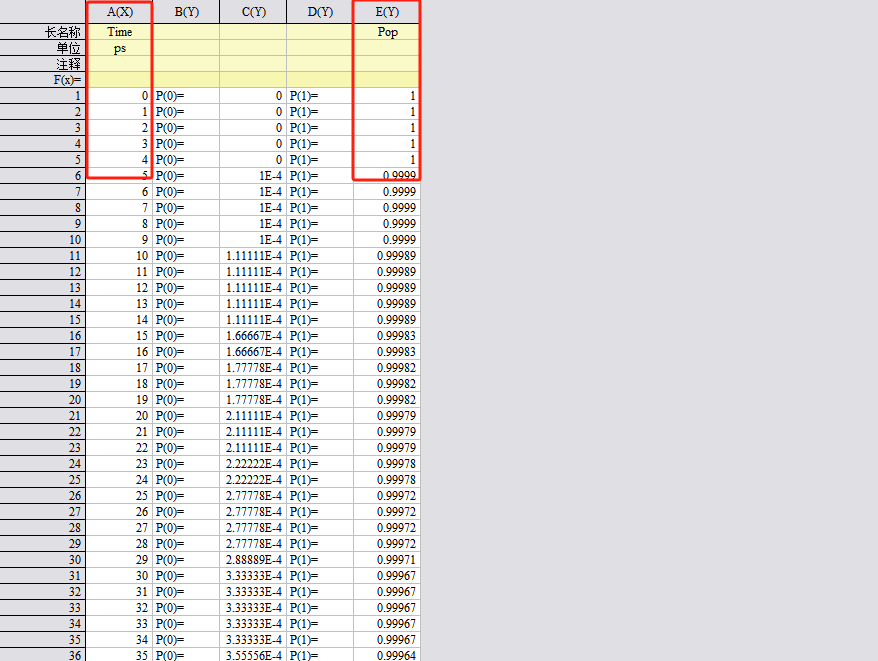
pop.dat
绘制后应该是从1下降,斜率为K, -1/K为寿命(单位为 fs)
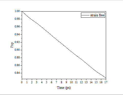
pop.img
要得到K,需要使用origin拟合斜率,y轴截距设置为1。
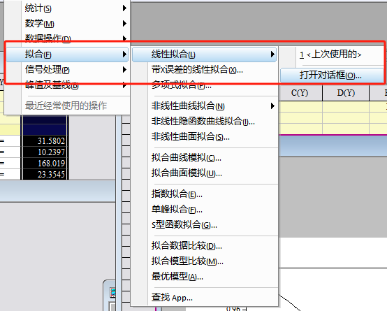
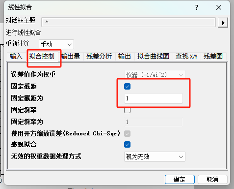 fit
fit
Dephasing:
退相干:
将icond0pair0_1Dephasing_function.txt的第一和第三列作为x和y导入origin,绘制图。
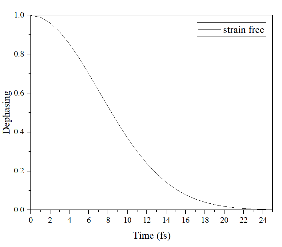 dephasing.img
认为下降到0.6就是Dephasing time(单位 fs)
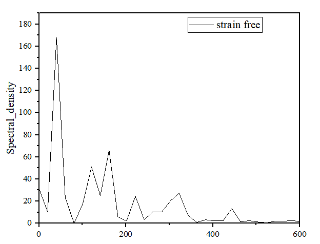
Spectral_density:
振动谱:
将icond0pair0_1Spectral_density.txt的第4列作为为x轴,第8列作为y轴)导入至origin,设置好x轴范围
附录
pyxaid2/PYXAID2 at master · Quantum-Dynamics-Hub/pyxaid2
Prof. Jin Zhao’s research group
Teaching | Prof. Jin Zhao’s research group(Solid State Phyics Course)